Overview
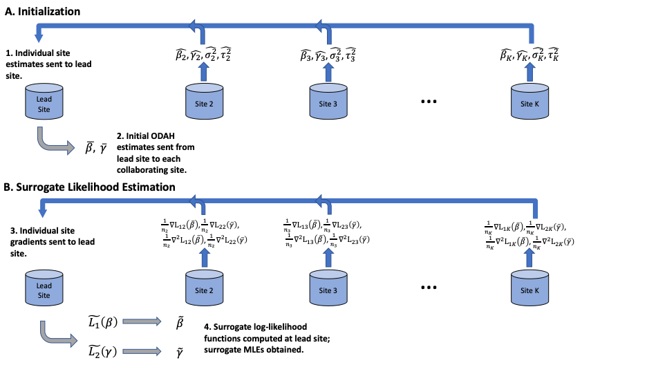
In a multicenter study, our ODAH algorithm allows researchers to fit a Poisson-Logit hurdle regression model across multiple data sets without needing to directly share subject-level information. The Poisson-Logit hurdle model is a two-part model for modeling zero-inflated count data, or counts with a larger proportion of zeros than would be expected in a traditional count data distribution (e.g. Poisson or Negative Binomial). Before conducting the multicenter analysis, all datasets need to be converted to a unified format where all the variables are defined in a standard way (e.g, OMOP Common Data Model). We require one of the sites to be the coordinating site, and the rest to be the participating sites. The coordinating site is responsible for obtaining and broadcasting the initial value of model parameters, synthesizing information obtained from other sites, and obtaining the final results. The participating sites only need to calculate the aggregated data and transfer them to the coordinating site. A more detailed description is provided below.
Poisson-Logit Hurdle Regression Model
Suppose we have K sites, and the coordinating site is the first site. For the i-th individual in the j-th site, we denote the count outcome to be \(y_{ij}\), and a vector of explanatory variables to be \(z_{ij}\). Let \(x_{ij} = (1, z_{ij}^{T})^T\). The hurdle regression model is a two-part model, consisting of a “zero” part and a “non-zero” part. The “zero” part is a logistic regressio model which assumes that
\(logit(Pr(y_{ij}=1)|x_{ij}) = x_{ij}^{T}\beta\)
where \(logit(t) = log\left \{ t/(1-t) \right \}\) and \(\beta\) is the vector of intercept and regression coefficients for the logistic component of the hurdle model. This models the probability that a particular count is non-zero. The “non-zero” part is a zero-truncated Poisson regression model which assumes that
\(P(Y_{i} = y_{i}|Y_{i}>0) = \frac{e^{-\lambda_{i}} \lambda_{i}^{y_{i}}}{(1-e^{-\lambda_{i}})y_{i}!}\) with \(log(\lambda_{i}) = X_{i}^{T}\gamma\)
where \(\gamma\) is the vector of intercept and regression coefficients for the zero-truncated Poisson component of the hurdle model.
Algorithm
Our algorithm has two steps:
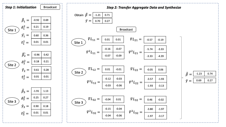
- First, each site fits a hurdle regression model using its own data and sends point and variance estimates from each component (logistic and zero-truncated Poisson) to the local site, where meta-analysis is done to compute initial estimates \(\bar{\beta}\) and \(\bar{\gamma}\). Initial estimates \(\bar{\beta}\) and \(\bar{\gamma}\) are then sent to all collaborating sites.
- Second, each collaborating site calculates first and second order gradients of their own likelihood functions (for each component) evaluated at the initial values \(\bar{\beta}\) and \(\bar{\gamma}\). These aggregate data are then transferred to the coordinating site, which combines these data with its own aggregate data to obtain \(\tilde{\beta}\) and \(\tilde{\gamma}\), improved estimates of \(\beta\) and \(\gamma\), respectively.

Figure 2 below gives an example of the information shared in each step in a setting with one explanatory variable in the model. For p explanatory variables, each site needs to transfer in total 2*((p+1) + p* (p+1)) numbers.

Sample code
Set the “control” in R as below to start ODAH algorithm
control <- list(project_name = 'CrabSatellites study',
                step = 'initialize',
                sites =  c('site1', 'site2'),
                heterogeneity = FALSE,
                model = 'ODAH',
                family = 'hurdle',
                outcome = "satellites",
                variables_hurdle_count = c("width", "weight"),
                variables_hurdle_zero = c("width", "weight"),
                offset = NULL,
                optim_maxit = 100,
                lead_site = 'site1',
                upload_date = as.character(Sys.time()) )
demo(ODAH)
